Hello and good day!
Today, I’m going to share with you how to calculate the most achievable profit for a production line of a company using the software: Microsoft Excel 2016.
To make my explanation easier for all of you, I will use an example of a business situation.
Situation:
The departments that can process either model by a company that produces a standard line and a deluxe line of dishwashers, the following time requirements (in minutes) apply.
The standard models contribute $20 each to profits and the deluxe models contribute $30 each. Because the company produces other items that share the resources used to make the dishwashers, the stamping machine is only available for 30 minutes per hour, on average. The production line for installing the motors is available 60 minutes per hour. There are two lines for wiring, so the availability is 90 minutes per hour.
1. Prepare your Excel spreadsheet
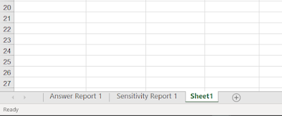
For this step, simply click on and open a spreadsheet in your Microsoft Excel 2016. The spreadsheet will look like the illustration above.
2. List the relevant factors, then transfer them to the spreadsheet.
From the situation, you can conclude several things:
1.) The topics we are focusing on. Here, the company’s product, the two types of dishwashers: standard and deluxe).
2.) The profit made by each of the products.
3.) The production information. (From the amount of resources available to the amount of resources that we use the following materials to produce each product).
) Plotting these on the worksheet will make the calculation process easier for you. You could say it’s like mind-mapping via Excel!
3. Define formulas on your worksheet
I marked the cells that need to have a formula in them. Now let me explain each of these cell areas.
- Usage (cells in the blue area)
The formula used is [B9*B14+C9*B15; B10*B14+C10*B15; B11*B14+C11*B15].
- Rest (cells in the red zone)
The formula used [F9-D9; F10-D10; F11-D11].
- Total profit (purple zone)
The formula used [B4*B14+C4*B15].
Adding formulas to your cells will make the calculations much easier. These formulas will automatically adjust all the data related to the calculations you have made.
4. Get to know Excel’s Solver function
Now you’re ready!
Now that you’ve made the adjustments to your spreadsheet, you can start tinkering with the Solver function. What is it? (For those unfamiliar with the function), Excel’s Solver function, or simply “Solver,” is a tool in Excel for calculating (or estimating) quick results of various scenarios of a situation.
However, the Solver is not available to Microsoft Excel 2016 users until they add the function manually.
Extra: Instructions for getting the Solver feature. Click File -> Option -> Add-ins -> Solver Add-in -> OK. (Keep in mind that these instructions are for Microsoft Excel 2016).
Once you have followed all the instructions, you will find the Solver in the “Data” tab.
5. Start calculating using the Solver function
To calculate or gain the result from the situation data, you must first open your Solver, and then adjust all the data factors on the function according to the situation.
The active Solver window is on the left.
- First, you need to adjust the target.
Click on the white insert area -> cell B17 (the cell in which you will place the profit data).
- Next, you need to set the To option.
Click on Max.
Why Max? Because you want to find the highest profit “maximize profit”.
- Next, insert the Constraints.
Click on Add.
The window above is a sub-window of the Solver. It is the window for adding constraint data to the current calculation. Just as you insert data in the aim section, you can also insert data in this section in the same way.
Following the addition of constraints, simply “check” the “Non-negative” statement, choose the “Simplex LP” solving method and click Solve!
6. Get the response and sensitivity report
The way we get these two reports reminds us how convenient Excel has made our work.
Using Excel, we will get these reports instantly by clicking on two things after clicking on “Solve” in the previous Solver window.
This other sub-window of the Solver will show you a few more options in what you can do after you finish your solving action.
All you have to do then is click on the report option you want to gain, in this case Response and Sensitivity -> Ok.
And that’s it!
Are you looking for the best and most powerful production planning software as an Excel spreadsheet that will allow you, as a planner, to deliver your goods on time? Then Scheduler123 is the perfect product that will meet all your needs.
Check https://deliverit.blogspot.com/p/production-planning-software.html for more details.
So those are all the things you can do if you want to calculate the highest profit available for a product line using Microsoft Excel 2016.
I hope this helps you out.
Thanks for reading!


